This is an old revision of the document!
Table of Contents
Amr Abdelkhalek (31309)
Irrigation Cart Nozzle
I. Introduction and Motivation
Water scarcity is an increasing global concern, necessitating the efficient use of available water resources. Traditional irrigation systems often waste significant amounts of water due to a lack of precise control over watering schedules; as can be demonstrated in the following video:


To address this issue, our target is to develop an automated irrigation cart nozzle system designed to water plants only when necessary, thus conserving water. This system uses sensor technology to detect the presence of plants and their specific needs, ensuring that water is used properly and sustainably.
II. Materials
Project Overview
In order to Simulate the Previous, a small primitive irrigation cart “Gießwagen” prototype was built. The project consists of the irrigation cart model equipped with two VL53L0X Time-of-Flight (ToF) sensors, an Arduino for sensor control and communication of the sensors' readings, and a Personal computer running Python Jupyter-Notebooks for data visualization and further processing. Communication between the Arduino and the laptop is facilitated via MQTT.
Components and Descriptions
The following table shows the general components needing for creating a single irrigating nozzle
Table 1: Components and Descriptions
| Component | Description |
|---|---|
| Arduino and VL53L0X Sensors | The Arduino microcontroller interfaces with two VL53L0X sensors to detect plant presence and monitor the movement of the irrigation cart. |
| LED-Licht | Acts as an alternative to the valve or the actuator that will be used to water the plant in the future. |
| Laptop with Python Jupyter Notebooks | Processes and visualizes data from the sensors, running Jupyter Notebooks for interactive analysis and decision making for the actuator. |
| Communication Protocol | MQTT is currently used for communication between the Arduino and the laptop, with possible exploration into WebSockets for improved performance. |
III. Methods and Implementation Details
Setup
The following diagram Figure 1 shows the overall layout of our project: the system uses LIDAR sensors for distance measurements, processes the data with an ESP32-S3-WROOM-1 microcontroller, and communicates the results to a personal computer and other components.
- VLX53L0X (LIDAR Sensors):
Horizontal Distance Input: One VLX53L0X sensor measures horizontal distance. Vertical Distance Input: Another VLX53L0X sensor measures vertical distance.
- ESP32-S3-WROOM-1 (Arduino):
Receives distance readings from both VLX53L0X sensors (horizontal and vertical distance). Processes these readings and performs various tasks based on the data.
- LED Light/Actuator:
Connected to the Arduino. Can be turned on or off based on commands from the Arduino.
- Battery/Charger:
Powers the ESP32-S3-WROOM-1.
- MQTT Server:
Receives processed readings (distance data and actuator state) from the Arduino. Sends actuator control commands (like “On” or “Off”) to the Arduino.
- Personal Computer with Jupyter Notebooks:
Communicates with the MQTT server to receive the distance readings and actuator state. control commands to the MQTT server, which then relays them to the Arduino.
The following Figure 2 is the implementation of the previous layout in real-life application:
 Fig. 2: Real-life Implementation
- Vertical VL53L0X Sensor
- LED-Licht
- Horizontal VL53L0X Sensor
- ESP32-S3-WROOM-1 Arduino
System Description
Sensor Setup
Two VL53L0X sensors are utilized in this system:
- Vertical Sensor: An upside down sensor to detect level difference on the ground which is used to detect changes in height to identify the presence of a plant.
- Horizontal Sensor: Monitors the lateral movement of the irrigation cart to ensure accurate positioning.
Functional Workflow
- Detection of Plant Presence: The vertical sensor identifies height changes. When the sensor detects a height above a certain threshold, it indicates the presence of a plant.
- Movement Tracking: The horizontal sensor tracks the cart's sliding movement to ensure it is correctly aligned with the plants.
- Watering Mechanism: Based on sensor data, the system decides when to activate or deactivate the water nozzle, ensuring water is only dispensed when a plant is present.
Arduino Code
The Arduino code handles data collection from the VL53L0X sensors and communicates with the laptop via MQTT. Below is an excerpt from the Arduino
The C++ code was used… please find the comments to clarify as steps proceed
- Two_TOFs_VL53L0X_Profiler_S3_Dev_publisher.ino
#include <Wire.h>
#include <WiFi.h>
#include <PubSubClient.h>
#include <Adafruit_VL53L0X.h>
#include <math.h>?>
// Toggle Debug Messages
bool debugOn = true;

// Set Interval
uint16_t hz = 10;

// Replace with your network credentials
const char* ssid = "SSID";
const char* password = "SSID_Password";

// Our MQTT Broker IP address
const char* mqtt_server = "test.mosquitto.org";
const char* my_client_id = "ESP32Client";

const char* my_mqtt_topic_sensor = "gw/duese002";
const char* my_mqtt_topic_actuator = "gw/duese002-licht";


// Setup WiFi client and MQTT client
WiFiClient espClient;
PubSubClient client(espClient);

// Set up an instance for each sensor
Adafruit_VL53L0X tof1 = Adafruit_VL53L0X();
Adafruit_VL53L0X tof2 = Adafruit_VL53L0X();

// Shutdown pins
#define SHT_TOF1 35 //32 in our older system
#define SHT_TOF2 40 //33 in our older system

// Sensor readings
uint16_t x = 0;
uint16_t z = 0;

// Define the data object for sensor measurement
VL53L0X_RangingMeasurementData_t measure1;
VL53L0X_RangingMeasurementData_t measure2;

unsigned long lastMsg = 0;

// LED Pins
const int dueseLedPin = 4;
const int OoRLedPin = 15; //25 in our older system

int sda_pin = 16; // GPIO16 as I2C SDA (Right_Blue Side on Board)
int scl_pin = 17; // GPIO17 as I2C SCL (Right_Red Side on Board)

void setup() {

  Wire.setPins(sda_pin, scl_pin); // Set the I2C pins before begin
  Wire.begin(); // join i2c bus (address optional for master)


  if (debugOn) Serial.begin(115200);

  setup_wifi();
  client.setServer(mqtt_server, 1883);
  client.setCallback(callback);

  pinMode(dueseLedPin, OUTPUT);
  pinMode(OoRLedPin, OUTPUT);

  digitalWrite(dueseLedPin, LOW);
  digitalWrite(OoRLedPin, LOW);

  pinMode(SHT_TOF1, OUTPUT);
  pinMode(SHT_TOF2, OUTPUT);

  digitalWrite(SHT_TOF1, LOW);
  digitalWrite(SHT_TOF2, LOW);

  delay(10);
  digitalWrite(SHT_TOF1, HIGH);
  delay(10);

  // Initialize sensor 1
  if (!tof1.begin(0x30)) {
    debug(F("Failed to boot VL53L0X - 01 (Vertical)"));
    while (1)
      ;
  }

  delay(10);
  digitalWrite(SHT_TOF2, HIGH);
  delay(10);

  // Initialize sensor 2
  if (!tof2.begin()) {
    debug(F("Failed to boot VL53L0X - 02 (Horizontal)"));
    while (1);
  }

  digitalWrite(SHT_TOF1, HIGH);
  digitalWrite(SHT_TOF2, HIGH);

  delay(10);
}

void loop() {
  if (!client.connected()) {
    reconnect();
  }
  client.loop();

  long now = millis();
  if (now - lastMsg > long(1000 / hz)) {  // Data transmission rate of 10Hz
    lastMsg = now;

    // Reading distance from both sensors
    tof1.getSingleRangingMeasurement(&measure1, false);
    if (measure1.RangeStatus != 4) {
      z = measure1.RangeMilliMeter;
       //Serial.print("Distance Vertical (mm): "); Serial.println(measure1.RangeMilliMeter);
    }

    tof2.getSingleRangingMeasurement(&measure2, false);
    if (measure2.RangeStatus != 4) {
      x = measure2.RangeMilliMeter;
      //Serial.print("Distance Horizontal (mm): "); Serial.println(measure2.RangeMilliMeter);

    }

    // Current time in milliseconds.
    long t = now;

    // Create data payload
    String payload = String("(") + String(t) + ", " + String(x) + ", " + String(z) + ")";

    // Publish data
    // Checks the readings noise-freeness; VL53L0X gives an output of 8191 by having so much noise by the environment
    if (x != 8191 && z != 8191 && x > 90 && z > 90) {
      digitalWrite(OoRLedPin, LOW);
      client.publish(my_mqtt_topic_sensor, (char*)payload.c_str());
      debug(payload);
    } else {
      digitalWrite(OoRLedPin, HIGH);
    }
  }
}

void setup_wifi() {
  delay(10);
  debug("");
  debug("Connecting to ");
  debug(ssid);

  WiFi.begin(ssid, password);

  while (WiFi.status() != WL_CONNECTED) {
    delay(500);
    debug(".");
  }

  debug("");
  debug("WiFi connected");
}

void reconnect() {


  //debug(F("Connecing to the MQTT server ..."));
  //debug(mqtt_server);

  while (!client.connected()) {

    if (client.connect(my_client_id)) {
      // Once connected, resubscribe to the required topic
      client.subscribe(my_mqtt_topic_actuator);
      //Serial.println("MQTT connected"); //state when successfully connected to the MQTT server
    }
    else {
      //Serial.print(client.state());
      //delay(5000);
    }

    debug(F(".."));
  }
}

void callback(char* topic, byte* message, unsigned int length) {
  String messageTemp;

  for (int i = 0; i < length; i++) {
    Serial.print((char)message[i]);
    messageTemp += (char)message[i];
  }

  // Feel free to add more if statements to control more GPIOs with MQTT

  // If a message is received on the topic esp32/output, you check if the message is either "on" or "off".
  // Changes the output state according to the message
  if (String(topic) == my_mqtt_topic_actuator) {
    if(messageTemp == "on"){
      digitalWrite(dueseLedPin, HIGH);
    }
    else if(messageTemp == "off"){
      digitalWrite(dueseLedPin, LOW);
    }
  }
}

void debug(String msg) {
  if (debugOn) {
    Serial.println(msg);
  }
}
Python Code
Required Libraries
To install the required libraries for the project, open and download the following text file “requirements.txt”
- requirements.txt
bqplot
traits
numpy
paho-mqtt
ipywidgets
pandas
Then run the following terminal command in the environment where you will run the project:
pip install -r requirements.txt
MQTT Client Setup and Configuration
# Setting the active MQTT broker address to "test.mosquitto.org"
BROKER = "test.mosquitto.org"


# Setting the active MQTT topic to "gw/duese002"
TOPIC = "gw/duese002"


# Setting the MQTT username
USER = "user"


# Setting the MQTT password
PW = "pw"


# Importing the paho-mqtt client library for MQTT communication
import paho.mqtt.client as mqtt


# Importing bqplot for creating interactive plots
import bqplot
import bqplot.pyplot as plt
from bqplot import LinearScale


# Importing ipywidgets for creating interactive widgets in Jupyter notebooks
import ipywidgets as widgets


import numpy as np
from IPython.display import display, clear_output


# Setting the MQTT callback API version to version 2
my_mqtt_api_ver = mqtt.CallbackAPIVersion.VERSION2
Creating an Output Widget for Displaying Decoded MQTT Messages
# Creating an output widget with a border layout
out = widgets.Output(layout={'border': '1px solid black'})


# Appending an initial message to the output widget
out.append_stdout('HERE THE DECODED MQTT MESSAGES WILL BE SHOWN!\n')
display(out)
Initializing Data and Plot for Plant Profile Scanner
# Initialize additional variables for data processing
i = 0
t0 = traw = t = x = z = 0
payload = ""
dx = 5 # mm
#N2 = 200

#N1 = 50
N1 = 870 # Number of data points


xsc_min = 0
xsc_max = 1000
ysc_min = 0
ysc_max = 500
xsc_margin = 20
ysc_margin = 20

x_acc = np.arange(xsc_min, xsc_max+1e-3, dx)  # Initialize with empty arrays
N2 = len(x_acc)
n_acc = np.array(np.zeros(N2))  # Initialize with empty arrays
z_acc = np.array(np.zeros(N2))  # Initialize with empty arrays
# Generate N1 linearly spaced data points between xsc_min and xsc_max to represent the x-axis values
x_data = np.linspace(xsc_min, xsc_max, N1)


# Initialize an array of zeros with length N1 to represent the z-axis values
z_data = np.array(np.zeros(N1))


# Initialize an array of zeros with length N1 to represent the t-axis (time) values
t_data = np.array(np.zeros(N1))


# Combine t_data, x_data, and z_data into a single array and transpose it to have the correct shape (N1, 3)
data = np.array([t_data, x_data, z_data]).T


# Update the first data set in the plotter with the combined data array
plotter.update_data1(data)


# Generate random data for the second data set, with values scaled by 1, 1000, and 500 for t, x, and z respectively
data2 = np.random.rand(N2, 3) * (1, 1000, 500)


# Update the second data set in the plotter with the generated random data
plotter.update_data2(data2)


# Clear the current plot by removing all data points from both scatter plots
plotter.clear()
PlantProfilePlot Class for Dynamic Data Plotting
The PlantProfilePlot class is designed to create a dynamic plot of plant profiles, updating the plot with new data in real-time. It leverages the HasTraits class from the traits library to observe changes in data and update the plot accordingly.
class PlantProfilePlot(HasTraits):
    # Import global variables to be used in the class
    global N1, N2, xsc_min, ysc_min, xsc_max, ysc_max, xsc_margin, ysc_margin


    # Create a figure for plotting with specified layout dimensions
    fig = plt.figure(layout=dict(height="600px", width="1200px"))

    # Define x and y scales for the plot, including margins
    x_scale = LinearScale(min=xsc_min - xsc_margin, max=xsc_max + xsc_margin)
    y_scale = LinearScale(min=ysc_min - ysc_margin, max=ysc_max + ysc_margin)


    # Initialize arrays to store data for plotting
    figdata1 = Array(shape=(N1, 3))  # Array for first scatter plot: columns are t, x, z
    figdata2 = Array(shape=(N2, 3))  # Array for second scatter plot: columns are t, x, z

    # Initialize empty scatter plots with specified colors and sizes
    scatter1 = plt.scatter([], [], colors=['red'], default_size=30, scales={'x': x_scale, 'y': y_scale})
    scatter2 = plt.scatter([], [], colors=['blue'], default_size=20, scales={'x': x_scale, 'y': y_scale})


    def __init__(self):
        super(PlantProfilePlot, self).__init__()
        # Initialize figdata arrays with random data scaled by max x and y values
        self.figdata1 = np.random.rand(N1, 3) * (1, xsc_max, ysc_max)
        self.figdata2 = np.random.rand(N2, 3) * (1, xsc_max, ysc_max)


    @observe("figdata1")
    def _on_figdata1_update(self, change):
        # Update scatter1 plot when figdata1 changes
        with self.scatter1.hold_sync():  # Disable automatic updates during this block
            if self.scatter1.x is not None:
                self.scatter1.x = self.figdata1[:, 1]
                self.scatter1.y = self.figdata1[:, 2]
            else:
                self.scatter1 = plt.scatter(self.figdata1[:, 1], self.figdata1[:, 2], colors=['blue'])


    @observe("figdata2")
    def _on_figdata2_update(self, change):
        # Update scatter2 plot when figdata2 changes
        with self.scatter2.hold_sync():  # Disable automatic updates during this block
            if self.scatter2.x is not None:
                self.scatter2.x = self.figdata2[:, 1]
                self.scatter2.y = self.figdata2[:, 2]
            else:
                self.scatter2 = plt.scatter(self.figdata2[:, 1], self.figdata2[:, 2], colors=['red'])


    def update_data1(self, new_data):
        # Method to update figdata1 with new data
        self.figdata1 = new_data


    def update_data2(self, new_data):
        # Method to update figdata2 with new data
        self.figdata2 = new_data


    def clear(self):
        # Method to clear both scatter plots
        self.scatter1.x, self.scatter1.y = [], []
        self.scatter2.x, self.scatter2.y = [], []


# Instantiate the PlantProfilePlot class and display the plot
plotter = PlantProfilePlot()
plt.show()
Initialize and Update Data Arrays for Plotting
# Generate N1 linearly spaced data points between xsc_min and xsc_max to represent the x-axis values
x_data = np.linspace(xsc_min, xsc_max, N1)


# Initialize an array of zeros with length N1 to represent the z-axis values
z_data = np.array(np.zeros(N1))


# Initialize an array of zeros with length N1 to represent the t-axis (time) values
t_data = np.array(np.zeros(N1))


# Combine t_data, x_data, and z_data into a single array and transpose it to have the correct shape (N1, 3)
data = np.array([t_data, x_data, z_data]).T


# Update the first data set in the plotter with the combined data array
plotter.update_data1(data)


# Generate random data for the second data set, with values scaled by 1, 1000, and 500 for t, x, and z respectively
data2 = np.random.rand(N2, 3) * (1, 1000, 500)


# Update the second data set in the plotter with the generated random data
plotter.update_data2(data2)


# Clear the current plot by removing all data points from both scatter plots
plotter.clear()

==== Defining and Initializing System States with Enum ====

class State(Enum):
    IDLE = 1       # State when the system is idle
    WATERING = 2   # State when the system is actively watering


# Initialize the current state of the system to IDLE
state = State.IDLE
MQTT Message Callback Function
on_message is a callback function to handle incoming MQTT messages. This function is called when a message is received from the MQTT broker.
The function processes the received message by decoding the payload, extracting the time, x, and z coordinates, updating the respective global variables and data arrays, and updating the plot and text widget with the new data.
Inputs:
- client: The MQTT client instance.
- userdata: Any user data (currently unused).
- message: The MQTT message containing the payload in the format “(traw, xraw, zraw)”.
Outputs:
- Unordered List Item The function updates global variables and UI elements but does not return any value.
def on_message(client, userdata, message):
    global payload, plotter, out
    global i, t, t0, x, z, traw, xraw, zraw
    global t_data, x_data, z_data
    global n_acc, x_acc, z_acc
    global state


    # Parse the received message
    payload = message.payload.decode('utf-8')  # Decode the message payload from bytes to a string
    traw, xraw, zraw = map(float, payload.strip('()').split(','))  # Parse the payload string and convert to floats


    # Initialize t0 on the first message
    if i == 0:
        t0 = traw  # Set the initial time value


    # Calculate the relative time and positions
    t = traw - t0  # Calculate the elapsed time since the first message
    x = x0 - xraw  # Calculate the x position relative to the initial x0
    z = z0 - zraw  # Calculate the z position relative to the initial z0

    # Format the parsed values into a string
    s = f"{i:4d}  {t:12.2f}  {x:6.2f}  {z:6.2f}"


    # Control logic based on state and z value
    if state == state.IDLE and z > 120:
        client.publish("gw/duese002-licht", "on")  # Publish "on" command if z > 120 and in IDLE state
        state = state.WATERING  # Update state to WATERING
    elif state == state.WATERING and z < 100:
        client.publish("gw/duese002-licht", "off")  # Publish "off" command if z < 100 and in WATERING state
        state = state.IDLE  # Update state to IDLE

    i += 1  # Increment the message counter


    # Update the data arrays by shifting and adding the new values
    t_data = np.roll(t_data, -1); t_data[-1] = t  # Shift t_data left and insert new t value
    x_data = np.roll(x_data, -1); x_data[-1] = x  # Shift x_data left and insert new x value
    z_data = np.roll(z_data, -1); z_data[-1] = z  # Shift z_data left and insert new z value

    data = np.array([t_data, x_data, z_data]).T

    plotter.update_data1(data)
    # Update the scatter plot with the new data


    # Calculate the index in x_acc closest to x
    idx = int(np.round(x / dx))


    # Update z_acc based on the calculated index
    if 0 <= idx < N2:
        if n_acc[idx] == 0:
            z_acc[idx] = z
        else:
            z_acc[idx] = (4 * z_acc[idx] + z) / 5  # Update z_acc with a moving average formula


        n_acc[idx] += 1  # Increment the counter for the corresponding x_acc index


    data2 = np.array([n_acc, x_acc, z_acc]).T  # Prepare data for updating plotter with n_acc, x_acc, z_acc


    plotter.update_data1(data)  # Update plotter's first data set
    plotter.update_data2(data2)  # Update plotter's second data set
MQTT Client Connection Callback Function
It is a callback function to handle MQTT client connection events.
Parameters
- client: paho.mqtt.client.Client
- The MQTT client instance that is calling the callback.
- userdata: any
- The private user data as set in Client() or userdata_set(). This parameter is currently not used in this function.
- flags: dict
- Response flags sent by the broker.
- rc: int
- The connection result code. This parameter indicates the success or failure of the connection attempt.
- 0: Connection successful
- 1: Connection refused - incorrect protocol version
- 2: Connection refused - invalid client identifier
- 3: Connection refused - server unavailable
- 4: Connection refused - bad username or password
- 5: Connection refused - not authorized
- 6-255: Currently unused.
- callback_api_version: int
- An extra unused argument to count for the API version an avoid an error in the case of selecting client_ID.
def on_connect(client, userdata, flags, rc,  callback_api_version):


    # Print the connection result code to the console
    print("Connected with result code " + str(rc))


    # Append the connection result code to the output widget
    out.append_stdout("Connected with result code " + str(rc) + "\n")
MQTT Client Configuration and Connection Setup
# Create an MQTT client instance with the specified callback API version
client = mqtt.Client(callback_api_version=my_mqtt_api_ver)


# Assign the on_connect function to handle connection events
client.on_connect = on_connect
# Assign the on_message function to handle incoming messages
client.on_message = on_message

#client.username_pw_set(USER, PW)   #if it needed any

# Connect to the specified MQTT broker
client.connect(BROKER, 1883, 60)


# Subscribe to the specified MQTT topic
client.subscribe(TOPIC)


# Start the MQTT client loop in the background
client.loop_start()
While also allows the program to react directly as soon as it receives the readings to publish back if the water.state should be on or off (because of the on_message function)
IV. Results of the first implementation
Simulation of the system
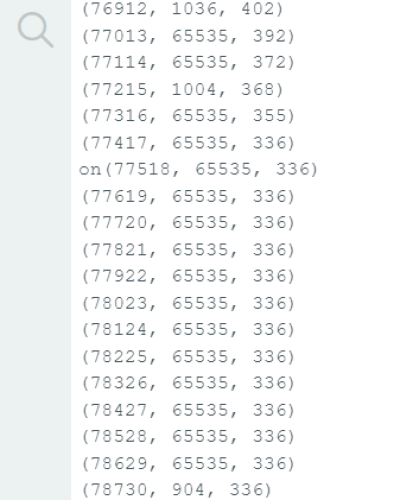
The simulation just as expected from our code, it senses height and accordingly sets the LED-licht “on” as a plant higher than the 120 mm is present, while it turns “off” as the height drops below 100 mm
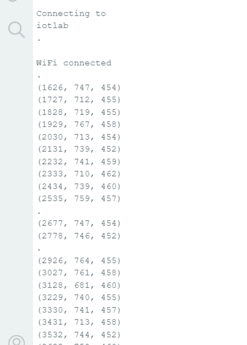
Arduino Code Output
After activating the Serial Monitor from the tools bar in the arduino IDE just as expected: the wifi connection is set and the output is displayed exactly as it would be published via the MQTT in the format (t , x , z)
where t is time, x is the horizontal distance to the wall, and z is the vertical distance from the surface
V. Discussion
Arduino Code Output Issues
- WiFi connection: An Antenna has to be used on the arduino to connect to the wifi for better connection as each of this point indicates a struggle to connect to the internet by the microcontroller
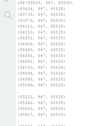
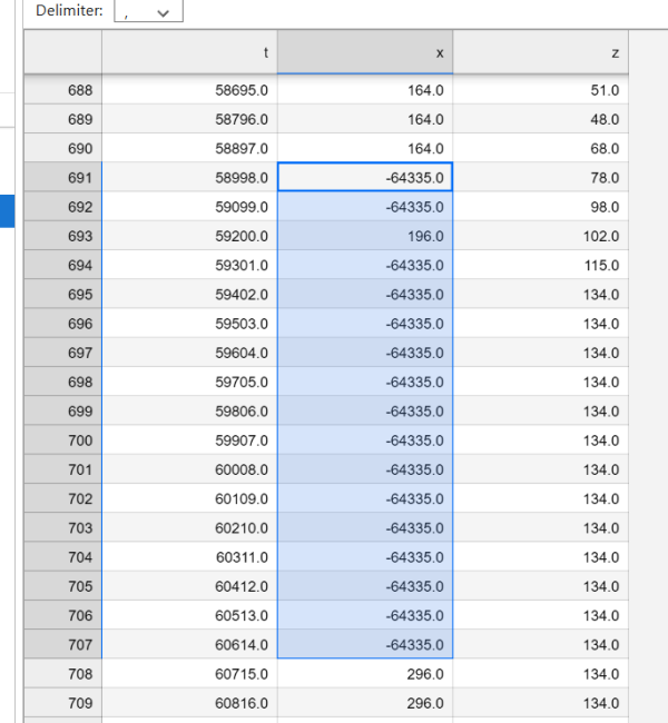
- Timeouts: rarely, but not never, does it happen where an output of exactly 65535 is displayed by one of the two vl53l0x sensors as shown in the next figure
This results from a timeout during the serial communication … the Arduino after exceeding the default is the one that creates this output of 65535 which is equal to (0xffff, 16 bits or 216) - 1 which is an unsigned 16 bit (0-65535) at full.
tackling this issue might lie in resetting the timeout value and the measurement time budget … please find more elaboration on this in the following github code https://github.com/pololu/vl53l0x-arduino/blob/master/examples/Single/Single.ino
Enhancing Plant Detection - Required
The first trial was successful where we were able to establish the communication between the microcontroller with the sensors and our personal computer. We were able to respond to the readings from the sensors through the laptop and back to the Arduino where it turned the LED on. Any plant above a threshold height of 120 mm was detected and irrigated and then it turned off when there was nothing. This already saves a lot of the excessive watering originally planned to be saved.
However this does not fix the problem of not turning the water on if there is simply noise of an obstacle above that same threshold existing temporarily on the track.
Ideally there would be a way to distinguish between actual plants and other objects with similar heights or even pick up shorter plans.
Enhancing Plant Detection - 2nd Implementation
To improve plant detection, it is crucial to distinguish between actual plants and other objects with similar heights. The following Python Jupyter Notebook implements another method to detect peaks representing plants, ensuring more accurate identification.
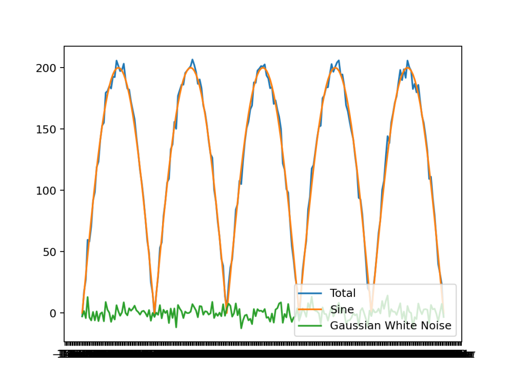
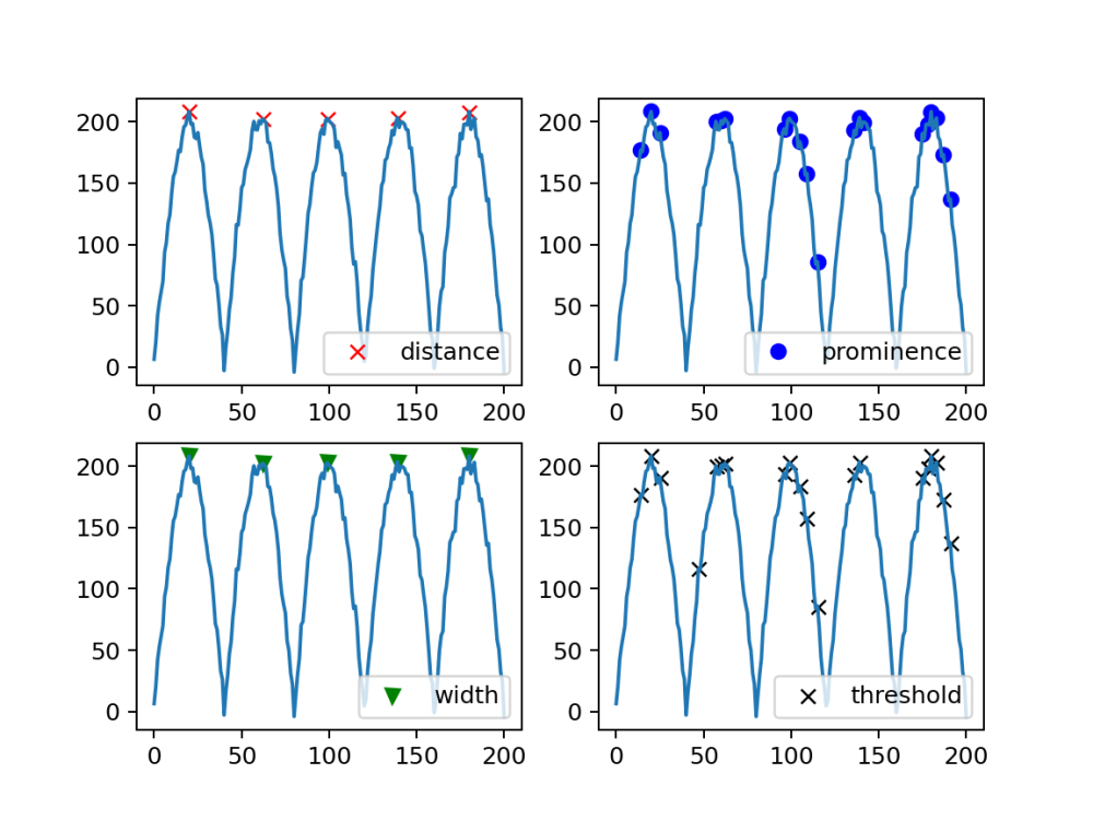
To test the peaks detection a sinusoidal plot with noise were plotted and the detection was tested on them:
Import necessary libraries
import numpy as np
from numpy import arange, pi, sin, abs
import time
import pandas as pd
import matplotlib.pyplot as plt
import ipywidgets as widgets
from IPython.display import display, clear_output
from matplotlib.ticker import FuncFormatter, MultipleLocator


# Import VBox and HBox for arranging widgets vertically and horizontally
from ipywidgets import VBox, HBox


  # Import find_peaks function from scipy for peak detection in signals
from scipy.signal import find_peaks
Sinusoidal function with clipping
A clipped sin wave that only has positive values used to simulate a plant detection like plot
def f(x, A=1, X=400, x0=0):


    # compute the sinusoidal function
    y = abs(A*sin(2*pi*1/X*(x-x0)))


    # clip negative values to zero #unnecessary line but just to ensure
    y[y<0] = 0


    return y
Noisy peaks generation
# Set the standard deviation for a normal distribution noise
STDDEV = 5.0


# Generate an array of x values from 0 to 1000 in steps of 5
x = arange(0, 1000.1, 5)


# Compute a sinusoidal function with amplitude 200, period 400, and phase shift 0
y = f(x, A=200, X=400)


# Determine the length of the x array
N = len(x)


# Generate Gaussian white noise with mean 0 and standard deviation STDDEV
noise_y = np.random.normal(0, STDDEV, N)


# Add the generated noise to the sinusoidal function to create a noisy signal
ys_noisy = y + noise_y


# Plotting
plt.Figure(figsize=(10, 6), dpi=80)  # Create a figure with specified size and dpi
plt.plot(x, ys_noisy, label='Total')  # Plot the noisy signal
plt.plot(x, y, label='Sine')  # Plot the clean sinusoidal signal
plt.plot(x, noise_y, label='Gaussian White Noise')  # Plot the generated noise

# Get the current axis
ax = plt.gca()
ax.xaxis.set_major_formatter(FuncFormatter(lambda val, pos: '{:.0f}$\pi$'.format(val / np.pi) if val != 0 else '0'))
ax.xaxis.set_major_locator(MultipleLocator(base=np.pi))

plt.legend(loc='lower right') # Display legend
plt.savefig("noisy_sine.png", dpi=180)  # Save the plot as an image file
plt.show()  # Display the plot
Peak Detection with Various Parameters Using find_peaks
our sin generated Array with noise was then put into the find_peaks function in SciPy
Please find a clear overview over the documentation of this library and its parameters in the following link https://docs.scipy.org/doc/scipy/reference/generated/scipy.signal.find_peaks.html#scipy.signal.find_peaks
These Parameters were played with a bit to find which arguments needed to be used for our specific application
#Find peaks using different parameters and store the indices of peaks
peaks, _ = find_peaks(ys_noisy, distance=20)
peaks2, _ = find_peaks(ys_noisy, prominence=1)
peaks3, _ = find_peaks(ys_noisy, width=25)
peaks4, _ = find_peaks(ys_noisy, threshold=0.4)

# Plotting each set of detected peaks
plt.subplot(2, 2, 1)
plt.plot(peaks, ys_noisy[peaks], "xr"); plt.plot(ys_noisy); plt.legend(['distance'],loc='lower right')
plt.subplot(2, 2, 2)
plt.plot(peaks2, ys_noisy[peaks2], "ob"); plt.plot(ys_noisy); plt.legend(['prominence'],loc='lower right')
plt.subplot(2, 2, 3)
plt.plot(peaks3, ys_noisy[peaks3], "vg"); plt.plot(ys_noisy); plt.legend(['width'],loc='lower right')
plt.subplot(2, 2, 4)
plt.plot(peaks4, ys_noisy[peaks4], "xk"); plt.plot(ys_noisy); plt.legend(['threshold'],loc='lower right')


plt.savefig("find_peaks_comparison.png", dpi=180)  # Save the plot as an image file
plt.show()
Testing on Real Data
Real Data had to be generated and saved for an extensive testing on them and they had to be the same readings through the multiple tests (to act as a control sample)
Real data generation and saving
Global variable data was added the other defined variable in the on_message function
def on_message(client, userdata, message):
    global payload, plotter, out
    global i, t, t0, x, z, traw, xraw, zraw
    global t_data, x_data, z_data
    global n_acc, x_acc, z_acc
    global state

    global data # as can be seen here
Then that data array was used after having many real readings after a visit to the lab
dataset = pd.DataFrame({'t':  t_data, 'x':  x_data,'z':  z_data}, columns=['t', 'x','z'])
dataset.set_index('t', inplace=True)

dataset.to_csv("./sample_txz.csv")
the array were turned into a pandas dataframe then saved as a CSV file for later use
Data Loading, Preprocessing, and Filtering
# Load dataset from CSV file into a pandas DataFrame
RealDataSet = pd.read_csv('sample_txz.csv')


# Extract 'z' and 'x' columns from the DataFrame and convert them to NumPy arrays
array_z = RealDataSet[['z']].to_numpy()
array_x = RealDataSet[['x']].to_numpy()


# Example of accessing the last element in array_z
array_z[len(array_z)-1]


# Get the shape of array_z
array_z.shape


# Remove singleton dimensions from array_z
np.squeeze(array_z).shape


# Squeeze the array_z to remove singleton dimensions
array_z = np.squeeze(array_z)
array_x = np.squeeze(array_x)


# Get the shape of array_z after squeezing
array_z.shape


# Set values in array_z and array_x to 0 if they are greater than 1000 or less than 0
array_z[(array_z > 1000) | (array_z < 0)] = 0
array_x[(array_x > 1000) | (array_x < 0)] = 0
The last function dealt temporarily with the timeout 65535 values from the Arduino … which were saved as a large negative value due to the following two functions:
x = x0 - xraw
z = z0 - zraw
in the on_message function
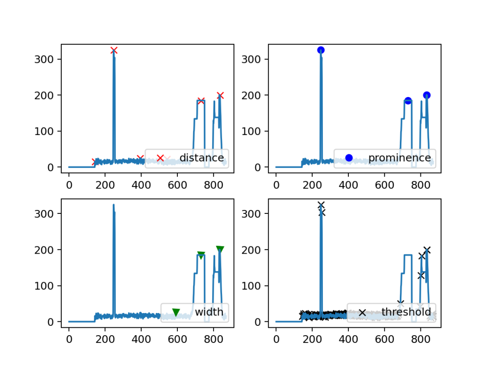
Trial 1:
# Plotting peaks detected in array_z using different parameters with find_peaks
peaks, _ = find_peaks(array_z, distance=100)
peaks2, _ = find_peaks(array_z, prominence=100)
peaks3, _ = find_peaks(array_z, width=25)
peaks4, _ = find_peaks(array_z, threshold=0.4)
# Plotting each set of detected peaks
plt.subplot(2, 2, 1)
plt.plot(peaks, array_z[peaks], "xr"); plt.plot(array_z); plt.legend(['distance'],loc='lower right')
plt.subplot(2, 2, 2)
plt.plot(peaks2, array_z[peaks2], "ob"); plt.plot(array_z); plt.legend(['prominence'],loc='lower right')
plt.subplot(2, 2, 3)
plt.plot(peaks3, array_z[peaks3], "vg"); plt.plot(array_z); plt.legend(['width'],loc='lower right')
plt.subplot(2, 2, 4)
plt.plot(peaks4, array_z[peaks4], "xk"); plt.plot(array_z); plt.legend(['threshold'],loc='lower right')


plt.savefig("Real_find_peaks_comparison.png", dpi=180)  # Save the plot as an image file
plt.show()
Worthy to mention that the extreme peak at the beginning is myself being close to the sensor to simulate a bird passing by or any presence of noise to the readings
Trial 2:
# Now try the prominence and the threshold parameters together in the find_peaks function
peaks2, prm = find_peaks(array_z, prominence=100,threshold=0.2)


plt.plot(peaks2, array_z[peaks2], "ob"); plt.plot(array_z); plt.legend(['prominence'],loc='lower right')


# Save the plot as an image file
plt.savefig("find_peaks_prominence.png", dpi=180)


plt.show()
using prominence is similar to using a vertical threshold such as the one we used in our earlier code (120 mm) but cleaner and fancier.. despite using distance which can help us clear a little bit of the horizontal noise in the case of the sensor reading multiple times the same plant over the same place it still would not get rid of vertical noise such as myself which was indicate by the first peak being detected … and if an upper bound of prominance would to be used this may create a problem later when the plants grow to greater heights.
The risk of using large distances can have the risk of ignoring another “real” plant if not watched out for .. as clearly seen with the second peak which actually is a real plant
Trial 3
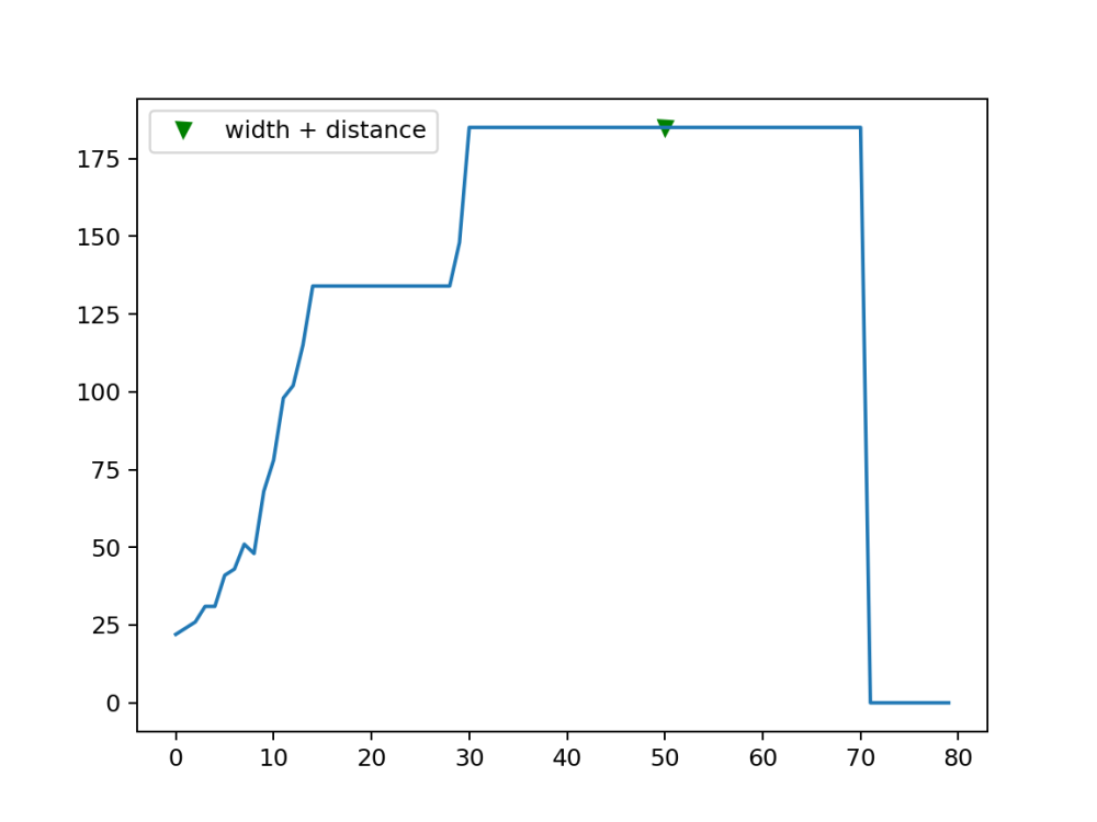
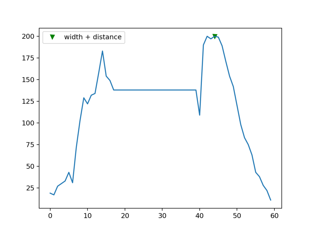
Using Width seems to be the more reasonable choice for our application as it allows us to detect our proper peaks while mixing this with distance makes us able to identify different plants as many peaks can appear and turn out to be for the same plant .. as would actually come if we don't use the distance argument for our next example. The also perfect part about it is that all it needs is just the lower readings on both sides of the peak … which would allow us to pick a single plant if needed as will be demonstrated in the following:
array_z_sample = array_z[680:760] selected one of the peaks

peaks5, wid_dis = find_peaks(array_z_sample, width=9,distance=50)
plt.plot(peaks5, array_z_sample[peaks5], "vg"); plt.plot(array_z_sample); plt.legend(['width + distance'])
plt.savefig("Peak1_wid_dist.png", dpi=180)  # Save the plot as an image file


array_z_sample = array_z[790:850] #2nd Peak

peaks5, wid_dis = find_peaks(array_z_sample, width=9,distance=50)
plt.plot(peaks5, array_z_sample[peaks5], "vg"); plt.plot(array_z_sample); plt.legend(['width + distance'])
plt.savefig("Peak2_wid_dist.png", dpi=180)  # Save the plot as an image file
It produces the same peaks with the whole array of course
peaks5, wid_dis = find_peaks(array_z, width=9,distance=50)
plt.plot(peaks5, array_z[peaks5], "vg"); plt.plot(array_z); plt.legend(['width + distance'])
Analysing the peaks using the find_peaks parameters
This allows us to use these peaks with the output information produced by the find_peaks so that we can analyse the peaks save them and with the possibility to save them in files and/or in online databases
peaks5, wid_dis = find_peaks(array_z, width=9,distance=50)
plt.plot(peaks5, array_z[peaks5], "vg"); plt.plot(array_z); plt.legend(['width + distance'])
wid_dis
{'prominences': array([179., 195.]),
 'left_bases': array([544, 774], dtype=int64),
 'right_bases': array([751, 859], dtype=int64),
 'widths': array([59.60878378, 42.81158358]),
 'width_heights': array([ 95.5, 102.5]),
 'left_ips': array([690.875     , 797.98387097]),
 'right_ips': array([750.48378378, 840.79545455])}
the left and right bases produced by the distance parameter … would allow us to integrate the peaks as demonstrated next:
#peak_no_integ.
peak_no = 2
lower_lat = wid_dis['left_bases'][peak_no-1]
upper_lat = wid_dis['right_bases'][peak_no-1]
np.trapz(array_z[lower_lat:upper_lat])
which gives an area under the peak value of about 7500 unit area
This can prove to be a very useful approach to keep track of the plants growth and health as the area of their peaks may prove to say a lot about their condition.
peaks5, wid_dis = find_peaks(array_z, width=9,distance=50)
i = 0
intg_peaks = np.array(np.zeros(len(peaks5)))
plant_name = np.array(np.zeros(len(peaks5)))
for peak in peaks5:
    peak_no = i
    lower_lat = wid_dis['left_bases'][peak_no]
    upper_lat = wid_dis['right_bases'][peak_no]
    integ_ea_peak = np.trapz(array_z[lower_lat:upper_lat])
    #np.append(intg_peaks, integ_ea_peak, axis=None)
    intg_peaks = np.roll(intg_peaks, -1); intg_peaks[-1] = integ_ea_peak

    i+=1
    plant_name = np.roll(plant_name, -1); plant_name[-1] = 10000 + i #row 1 is called 10000
intg_peaks #output the array of integrals of all peaks detected
array([12427.5, 7500.5])
Final Output
Using all the previous we can have a very good overview on the plants, their real position, their state, their real heights, and automatically naming them:
array_x[peaks5] #Horizontal position in mm of those found peaks
array([296., 253.])
And arranging all of them together in a pandas dataframe:
plant_dataset = pd.DataFrame({'plant_name':  plant_name, 'plant_position':  array_x[peaks5],'plant_height':  array_z[peaks5],'plant_peak_intg':  intg_peaks}, columns=['plant_name', 'plant_position','plant_height','plant_peak_intg']).set_index('plant_name')
plant_dataset.to_csv("../CSV_files/plants.csv")
plant_dataset
plant_name    plant_position	plant_height	plant_peak_intg

  10001.0	  296.0	             185.0	    12427.5
  10002.0	  253.0	             200.0	    7500.5
Enhancing the If-Condition for Better Plant Recognition
To enhance the condition for recognizing plants more accurately, we need to implement peak detection logic and replace the older one; to ensure only true plants are detected. This approach reduces the likelihood of false positives caused by objects with heights above 120 mm even as mentioned earlier and help creating an automated system that keeps track of the plants.
Enhancing the If-Condition for Better Plant Recognition
To enhance the condition for recognizing plants more accurately, we need to implement peak detection logic and replace the older one; to ensure only true plants are detected. This approach reduces the likelihood of false positives caused by objects with heights above 120 mm even as mentioned earlier and helps create an automated system that keeps track of the plants.
In order to implement this, testing the time required to detect plants' peaks through a full array by find_peaks is crucial.
This was tested on our array of 870 elements detecting the two peaks by the following line of command in the peak detecting step:
# Measure the time taken to find peaks in the array
%%time  #outputs the processing time

# Find peaks in the array 'array_z' with a specified width and distance between peaks
peaks5, wid_dis = find_peaks(array_z, width=9,distance=50)
CPU times: total: 0 ns
Wall time: 0 ns
# Note: The processing time changes if we have to plot every time, which in our application, we used the faster bqplot modules, but regardless:
# Measure the time taken to find peaks in the array
%%time #outputs the processing time

# Find peaks in the array 'array_z' with a specified width and distance between peaks
peaks5, wid_dis = find_peaks(array_z, width=9,distance=50)

# Plot the original data with the detected peaks
 plt.plot(peaks5, array_z[peaks5], "vg")
 plt.plot(array_z)
 plt.legend(['width + distance'])
CPU times: total: 15.6 ms
Wall time: 55.1 ms
but
# Measure the time taken to plot the results
%%time #outputs the processing time

# Plot the original data with the detected peaks
plt.plot(peaks5, array_z[peaks5], "vg");
plt.plot(array_z);
plt.legend(['width + distance'])
CPU times: total: 15.6 ms
Wall time: 54.4 ms
Confirming that all the time spent is in plotting and not searching for the peaks…this suggests that we can use find_peaks every reading or almost as often without worrying about spamming our hardware.
This was tested with our older real data:
# Initialize the arrays and variables for testing with our older real data

N1 = 870                              # Number of elements in the array
z_data = np.array(np.zeros(N1))       # Initialize with empty arrays (to resemble the variable we have in our on_message function)
peaks_total_xposition = np.array([])  # Initialize with empty array
peaks_last = np.array([])             # Initialize with empty array
counter = 0                           # Counter to keep track of the number of readings
counter_2 = 0                         # Secondary counter to keep track of the number of readings
checker = N1 / 10                     # Set to check 10 times every time the z_data array is completely filled
# Now check the output and the time of using this in a for-loop that activates for every reading to model our on_message function
%%time # Outputs the processing time
# Iterate through each element in array_z
for i in  array_z:
    # Shift the array to the left by one position
    z_data = np.roll(z_data, -1); z_data[-1] = i # Update the last element with the current reading
    counter += 1   # Increment the counter
    counter_2 += 1 # Increment the counter
    if counter == checker:
        # Find peaks in the z_data array with a specified width and distance between peaks
        peaks_wd, wid_dis = find_peaks(z_data, width=9,distance=50)
        if   len(peaks_wd) > len(peaks_last):
        # If the number of detected peaks is greater than the last detected peaks which indicates a new peak ...
            # Update the total x positions of the peaks
            # np.append(peaks_total_xposition, array_x[peaks_wd]): Append the current peak positions (array_x[peaks_wd]) to the existing peak positions (peaks_total_xposition)
            # np.unique(...): Remove duplicate peak positions from the appended array
            # np.sort(...): Sort the peak positions in ascending order
            peaks_total_xposition = np.sort(np.unique(np.append(peaks_total_xposition, array_x[peaks_wd])))
            peaks_last = peaks_wd # Update the last detected peaks
            counter = 0 # Reset the counter
    if counter_2 == N1:
        z_data = np.array(np.zeros(N1))    # Reset the z_data array
CPU times: total: 0 ns
Wall time: 35.8 ms
It may be a bit unnecessary to do the sorting unique check every time/reading for our peak detection array but again it worked. However, future optimization may be done here.
and the output was the same:
# Print the total x positions of the peaks
peaks_total_xposition
array([253., 296.]) # Output
Feel encouraged to compare with our last trial on the full array of array_z… it produces the same output
Structural adjustment by adding a lever
Adding a lever normal to the vertical axis of the cart aligned in the direction of the plants and attaching the vertical VL53L0X sensor to it… creates a lead from the vertical readings which in return would allow us to detect the peaks on spot and react to it just few centimetres later where the water nozzle and the rest of the cart is.
arm_sens_lead = 300 #mm
for i in  array_z:
    z_data = np.roll(z_data, -1); z_data[-1] = i
    counter += 1
    counter_2 += 1
    if counter == checker:
        peaks_wd, wid_dis = find_peaks(z_data, width=9,distance=50)
        if   len(peaks_wd) > len(peaks_last):
            # Calculate the new peak positions by adding the sensor lead distance to the current peak positions
            # np.full(len(array_x[peaks_wd]), arm_sens_lead): Creates an array of the same length as array_x[peaks_wd],
            # where every element is equal to arm_sens_lead (300 mm). This represents the lead distance for the sensor.
            # array_x[peaks_wd]: Retrieves the x positions corresponding to the detected peaks.
            # np.add(...): Adds the sensor lead distance to each of the x positions of the detected peaks.peak_positions =
            np.add(np.full(len(array_x[peaks_wd]), arm_sens_lead), array_x[peaks_wd])
            peaks_total_xposition = np.sort(np.unique(np.append(peaks_total_xposition,peak_positions)))
            peaks_last = peaks_wd
        counter = 0
    if counter_2 == N1:
       z_data = np.array(np.zeros(N1))
peaks_total_xposition
array([553., 596.])
Assuming the cart is 30 cm behind, then the values-added at this stage are also successful
Enhancing the If-Condition for Better Plant Recognition - Implementation
Now we will move to our on_message function and apply the new findings:
def on_message(client, userdata, message):
    global payload, plotter, out
    global i, t, t0, x, z, traw, xraw, zraw
    global t_data, x_data, z_data
    global n_acc, x_acc, z_acc , xsc_min, xsc_max
    global state
    global peaks_total_xposition, peaks_last
    global counter, counter_2, checker
    global arm_sens_lead

    global data

    # Parse the received message
    payload = message.payload.decode('utf-8')
    traw, xraw, zraw = map(float, payload.strip('()').split(','))

    if (i==0):
        t0 = traw

    t = traw - t0
    x = x0 - xraw
    z = z0 - zraw

    s = f"{i:4d}  {t:12.2f}  {x:6.2f}  {z:6.2f}"
    # Check if the system is idle and the current x position is at a peak position
    if (state == state.IDLE) & np.isin(x,peaks_total_xposition):# & (z > 120) if a threshold is needed
        client.publish("gw/duese002-licht", "on")
        state = state.WATERING
    # Check if the system is watering and the current x position is not at a peak position
    if (state == state.WATERING) & np.isin(x,peaks_total_xposition,invert=True):
        client.publish("gw/duese002-licht", "off")
        state = state.IDLE

     #checks if the water is off and the cart position is on a plant location .. turns it on
     #checks if the water is on and the cart position is not on a plant location (inverts the logic).. turns it off


    t_data = np.roll(t_data, -1); t_data[-1] = t
    x_data = np.roll(x_data, -1); x_data[-1] = x
    z_data = np.roll(z_data, -1); z_data[-1] = z

    data = np.array([t_data, x_data, z_data]).T

    counter += 1
    if counter == checker:
        peaks_wd, wid_dis = find_peaks(z_data, width=9,distance=50)
        if   len(peaks_wd) > len(peaks_last):
            peak_positions = np.add(np.full(len(x_data[peaks_wd]), arm_sens_lead), x_data[peaks_wd])
            peaks_total_xposition = np.sort(np.unique(np.append(peaks_total_xposition,peak_positions)))
            peaks_last = peaks_wd
        counter = 0

    if counter_2 == N1:
        x_data = np.linspace(xsc_min, xsc_max, N1)  # reinitialize with empty arrays
        z_data = np.array(np.zeros(N1))  # reinitialize with empty arrays
        t_data = np.array(np.zeros(N1))  # reinitialize with empty arrays

    plotter.update_data1(data)

# index of x_acc array with the x closest to x_acc[idx]
    idx = int(np.round(x/dx))
    if (idx >= 0) & (idx < N2):
        if n_acc[idx] == 0:
            z_acc[idx] = z
        else:
#            z_acc[idx] = (n_acc[idx] * z_acc[idx] + z) / (n_acc[idx] + 1)
            z_acc[idx] = (4 * z_acc[idx] + z) / 5

        n_acc[idx] += 1

    data2 = np.array([n_acc, x_acc, z_acc]).T

    plotter.update_data2(data2)

#    out.append_stdout(s + "\n")def on_message(client, userdata, message):
VI. Conclusion
This project addresses water scarcity by developing an automated irrigation cart that conserves water through precise plant detection and targeted watering.
Utilizing VL53L0X sensors and an Arduino, the system accurately monitors plant presence and cart movement, ensuring efficient water use.
The integration of MQTT for communication and Python for data processing lays the groundwork for future enhancements, including improved sensors and expanded scalability.
Future enhancements will focus on refining detection algorithms and exploring alternative communication protocols, including PostgreSQL Dashboards for reliable backups.
Sensors may be replaced in the future with faster detecting ones so that their algorithms may be easier or more straight forward to accommodate a much larger number of sensors.
Multiplexers most probably will be used for connecting with the multiple number of nozzles for our system e.g. irrigating 30 rows at the same time. Each of which will have at least a single sensor, and a water nozzle. 30 controlling MOSFETS hence may be connected to our microcontroller plus the 30 sensors.
Further studies are going to be done on the rush in current in case large nozzles will be used .. and 30 of those will mean multiple of that rush in current. Additionally, this further research will be conducted on managing current surges when using large nozzles might introduce the possibility of implementing PWM to ensure a smooth startup to mitigate the current spikes.
https://wiki.eolab.de/doku.php?id=eolab:projects:giesswagen:start
VII. References
- Pololu, “VL53L0X-arduino/examples/single/single.ino at master · Pololu/VL53L0X-arduino,” GitHub, https://github.com/pololu/vl53l0x-arduino/blob/master/examples/Single/Single.ino (accessed Jun. 17, 2024).
- “Find_peaks#,” find_peaks - SciPy v1.14.0 Manual, https://docs.scipy.org/doc/scipy/reference/generated/scipy.signal.find_peaks.html#scipy.signal.find_peaks (accessed Jul. 09, 2024).


